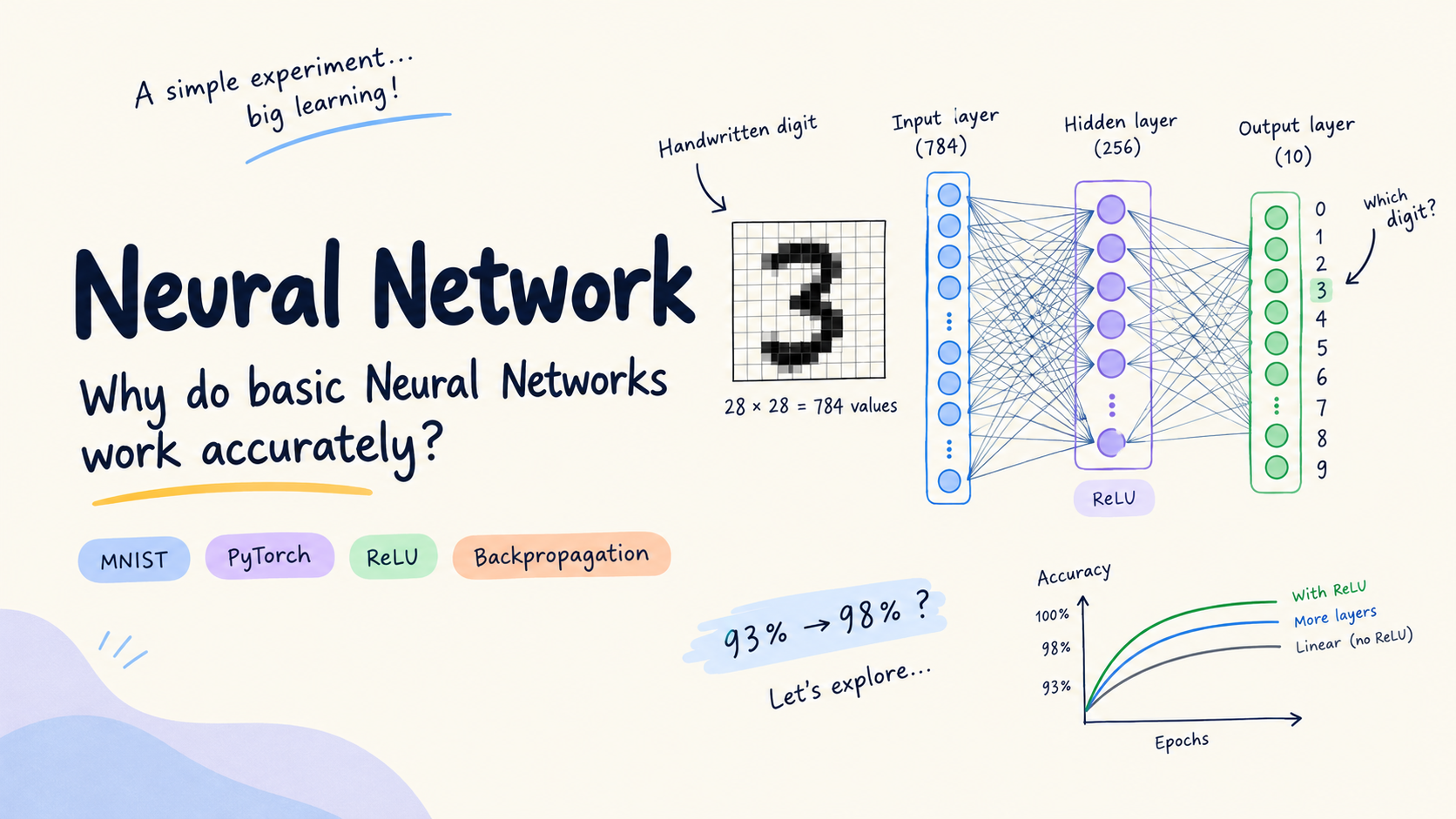
Neural Network
Natural Language / Image / Audio Processing are rising as major workloads along with traditional computations. So, Neural network architectures getting embedded into all software either directly or indirectly.
For end users interacting with any application, it offers simplicity. But software engineers working in this new era of products should know how things work underneath, to restructure themselves for the future.
Rather than explaining things, let's see a very small hands-on experiment which covers a basic Neural Network. Slightly longer post, bear with me.
Problem statement
To create a model recognizing the actual number written on paper.
For simplicity, instead of having picture of the digit as it is. We break it down as cells on grid with values corresponds to brightness.
Handwriting is made of free-flowing strokes. If we write the number in big checked (say grid) page, a number written goes via multiple cells to form the number. Since we handwrite the same, each way can cover different paths. A number 3 can be this and this.
A simplified view of the grid idea:
_ _ # # # _
_ _ _ _ # #
_ _ _ # # _
_ _ _ _ # #
_ _ # # # _
# represents a darker cell; _ represents a lighter cell. This is only a tiny conceptual example, not an actual MNIST image.


Pattern recognition of handwritten digits is the problem
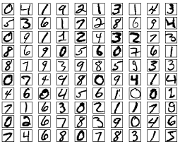
Fix the grid size as 28 × 28. Whichever cells the digit crosses, assume them as dark; the other cells are white. We now have 28 × 28 = 784 values between 0 and 1 for one handwritten digit as input. The expected output is one single number between 0 and 9.
Why 28 × 28? That's the classic MNIST dataset readily available\(^{[1]}\).
Input - 784 values of (0 ..., 1)
Output - 1 value in (0, 9)
Solution
- We will have layers. Input layer with 784 nodes. Output layer with nodes from 0 to 9.
- For a given number (784 cells as inputs). Each output node from 0 to 9 tries to provide a score. Whichever score is high, that is the answer.
- This is weird, right? If all nodes themselves guess a score, how come they are right.
Of course, they will be wrong if it guess. But, they maaaay beeeee, correct sometimes.
- If we replace the random function with exact example patterns function, the probability of having correct answer is more than pure random game. That may be is leveraged better and better. This is where the training starts.
- Next problem is how do we find function of example patterns. We don't have to. Instead of having different functions, we'll have different parameters for each node of same function. Each output node depends on all weights of input layer and some own param called bias.
- These different param values of each node using same function during forward pass of training and inference. Its called activation function. Here, we linearly add them as
sum of (weight * input) + bias.z = W x + b
Training process
Let's focus on the training process. We gave the input and the output nodes suggest a score using activation function.
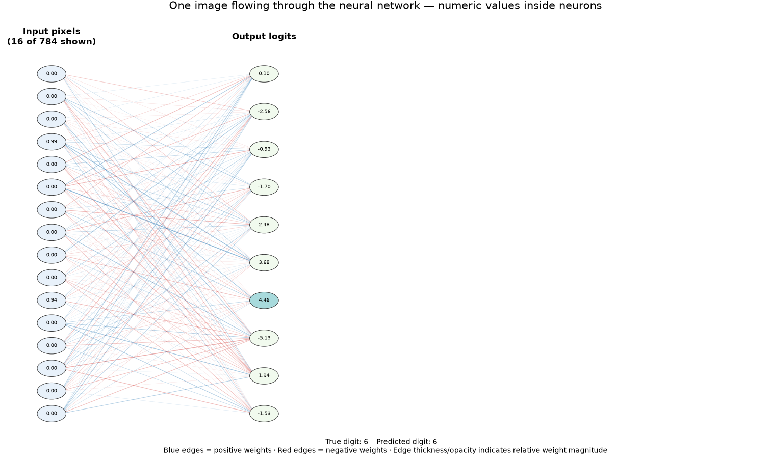
- Once we find a score during training, we compare it with the expected output. Then, we calculate how far the current prediction is from the expected output.
- The method of measuring this difference is called a
loss functioncalculation.Loss functionis a generic term. Implementation depends on the problem. Our example of Identifying digits comes under classification problem. One simple loss function for classification isCross-Entropy Loss. We have function now. - Our motive is to minimize the loss, i.e., to find its minimum. For a continuous function in mathematics, we use the slope to find the rate of change. In vector calculus, the gradient includes direction as well as magnitude. Since we need minimum loss, we use
Gradient Descent\(^{[3]}\) to update the parameters in the direction that reduces the loss. The goal is to find parameter changes that reduce the loss for the examples we train on. - Once the param changes are computed, we will update the model params respectively.
Since we have one output layer after input, we directly update the params of the model. If we have multiple hidden layers, we have to propagate the parameter updates through the layers. The process used to calculate how the loss changes with respect to parameters across the network is called backpropagation.
For each training example (or batch of examples), we do this process. Once the full training dataset has been processed, we repeat the process multiple times and validate against the validation data. One complete pass through the training dataset is called an epoch.
In the MNIST dataset\(^{[1]}\) we use, we have 50,000 training, 10,000 validation and test 10,000 data. We used only training and validation data in code.
It may not make sense, to accept that adjusting some parameter using known inputs and output create an AI model. Thats totally okay.
We humans derive solutions by rules and logics. So, it is weird. It took many decades\(^{[3]}\) arrive at the working model of the simple steps we discuss and much more than that for proper training. AI research faced multiple winters in funds and hope.
Let's see this example in code.
import pickle
from pathlib import Path

import torch
from torch import nn

"""
MNIST Dataset Citation

If you use this dataset or code in academic work, please cite:

@article{lecun2010mnist,
  title={MNIST handwritten digit database},
  author={LeCun, Yann and Cortes, Corinna and Burges, CJ},
  journal={AT&T Labs [Online]. Available: http://yann.lecun.com/exdb/mnist},
  volume={2},
  year={2010}
}
"""

path = Path("MNIST_dataset.pkl")

with path.open("rb") as f:
    data = pickle.load(f, encoding="latin1")

print("Type:", type(data))
(X_train, y_train), (X_val, y_val), (X_test, y_test) = data

# 1. Convert NumPy arrays to PyTorch tensors
X_train_t = torch.tensor(X_train, dtype=torch.float32)
y_train_t = torch.tensor(y_train, dtype=torch.long)

X_val_t = torch.tensor(X_val, dtype=torch.float32)
y_val_t = torch.tensor(y_val, dtype=torch.long)

# 2. Define a linear classifier
class MNISTModel(nn.Module):
    def __init__(self):
        super().__init__()
        self.linear = nn.Linear(784, 10)

    def forward(self, x):
        # Forward pass: Calculate 10 scores for every image
        return self.linear(x)

model = MNISTModel()

# Loss: Compare the scores with the correct labels. Cross-entropy penalizes incorrect predictions.
loss_fn = nn.CrossEntropyLoss()

# Optimizer: Update the weights to reduce the loss.
optimizer = torch.optim.SGD(model.parameters(), lr=0.1)

# 4. Train
batch_size = 128
epochs = 10

for epoch in range(epochs):
    model.train()

    # Shuffle the training examples each epoch
    indices = torch.randperm(len(X_train_t))
    total_loss = 0.0

    for start in range(0, len(indices), batch_size):
        batch_indices = indices[start:start + batch_size]

        images = X_train_t[batch_indices]
        labels = y_train_t[batch_indices]

        # Forward pass: make predictions
        logits = model(images)

        # Measure prediction error
        loss = loss_fn(logits, labels)

        # Backpropagation and weight update
        optimizer.zero_grad()
        loss.backward()
        optimizer.step()

        total_loss += loss.item() * len(batch_indices)

    # Evaluate on validation data
    model.eval()
    with torch.no_grad():
        val_logits = model(X_val_t)
        val_loss = loss_fn(val_logits, y_val_t).item()
        val_predictions = val_logits.argmax(dim=1)
        val_accuracy = (
            val_predictions == y_val_t
        ).float().mean().item()

    avg_train_loss = total_loss / len(X_train_t)

    print(
        f"Epoch {epoch + 1:2d} | "
        f"Train loss: {avg_train_loss:.4f} | "
        f"Val loss: {val_loss:.4f} | "
        f"Val accuracy: {val_accuracy:.2%}"
    )
Epoch   Train loss   Validation loss   Validation accuracy
    1       0.6149            0.3858                89.65%
   10       0.2986            0.2814                92.16%
   30       0.2700            0.2641                92.74%
   50       0.2601            0.2608                92.95%
   85       0.2509            0.2575                93.07%
  100       0.2482            0.2599                92.98%
 1000       0.2204            0.2731                92.70%
Increasing the number of epochs beyond 50 didn't help increase accuracy. In fact, 30 was good enough considering the maximum accuracy. That's it for the simple example.
Wait a minute. Can we increase the accuracy a bit?
Maybe it's possible with more training data. But we have a good amount of data to achieve 98 percent accuracy.
- We saw the small example and its code. Is there any definition of neural network model?
- Whats the model actually ?
Let's pause and ponder.
It's nothing but the values of the weights and biases we had. For each output node, we have (784 weights) and one bias. Multiply by 10 gives, we have 7850 parameters. These 7850 numbers stored as params helps us to classify the image. Thus, model is merely equal to what it have as parameters.
To increase the number of params, I shall add one hidden layer of 256 Nodes between input and output.
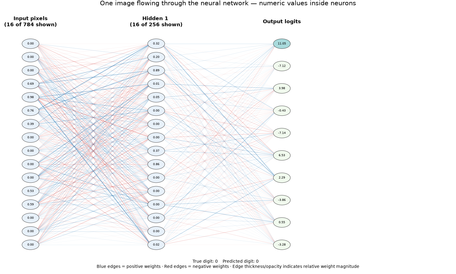
Now the param count = (784 * 256 + 256 * 10) + (256 + 10) = 203264 weights + 266 biases = 2,03,530 parameters model.
Let's try out the code again with new model.
class MNISTOneLayerModel(nn.Module):
    def __init__(self):
        super().__init__()

        self.hidden = nn.Linear(784, 256)
        self.output = nn.Linear(256, 10)

    def forward(self, x):
        x = self.hidden(x)   # 784 -> 256
        x = self.output(x)   # 256 -> 10
        return x


model = MNISTOneLayerModel()
OOPs. Not much improvements. Same 93 percent.
Epoch   Train loss   Validation loss   Validation accuracy
   30       0.2534            0.2627                92.97%
  100       0.2359            0.2691                92.87%
Non-Linearity is the key
If we look closely, we connected the new layer to the existing network as a linear function in the forward pass code.
Non-linearity is the key difference (ReLU activation step) between the two linear layers.

class MNISTOneLayerModel(nn.Module):
    def __init__(self):
        super().__init__()

        self.hidden = nn.Linear(784, 256)
        self.relu = nn.ReLU()
        self.output = nn.Linear(256, 10)

    def forward(self, x):
        x = self.hidden(x)   # 784 -> 256
        x = self.relu(x)
        x = self.output(x)   # 256 -> 10
        return x
Accuracy improved significantly (upto 98 percent), once we introduced non-linearity in the relationships.
Epoch   Train loss   Validation loss   Validation accuracy
   30       0.0351            0.0737                97.85%
  100       0.0044            0.0711                98.04%
This was the main surprise in my experiment: adding many more parameters alone did not help much, but adding ReLU made a clear difference.
Lets keep NN aside for a moment. In mathematics, linear functions are straight line. Non-linear functions can be curved or steps or straight line with bend. If multiple non-linear functions stacked together, it can form any shape.
Why shapes are important ?
Digit patterns and most of the world systems are continuous functions. We can split the large continuous function into many tiny non-linear functions (Eg. straight line with bend).
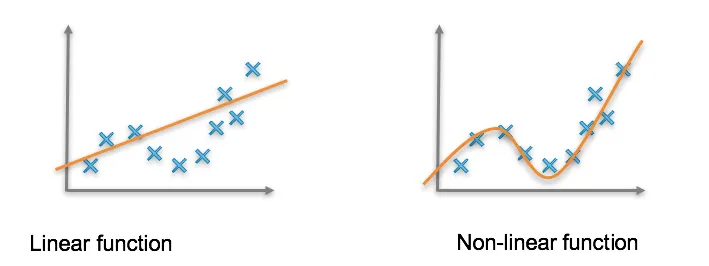
In Neural networks, intermediate nodes (neurons with activation function) are capable of capturing these tiny change in patterns across inputs and saving them.
Lets assume digit 3 has the pattern of three horizontal lines and two curves on right sides. Digit 5 also shares the top horizontal line with 3.
Intuition to start is nodes in hidden layers can capture the tiny patterns like common top line where the full forward pass can recognize the full pattern.
Idea of capturing complex patterns using many neurons is the basis for Universal Approximation Theorem\(^{[4]}\)
Note: Hidden layer capturing top line is oversimplified. But, idea of capturing tiny common patterns across inputs in hidden layers stays the same.
More Layers ...
When I tried to add one more and then two more hidden layers, here's what happened.
H-Layers Epoch   Train loss   Validation loss   Validation accuracy
      2     30       0.0077            0.0750               98.19%
      2    100       0.0005            0.0943               98.23%
      3     30       0.0013            0.0903               98.11%
      3.   100       0.0001            0.1119               98.09%
Even though we increase the number of layers, accuracy barely rises. Hence, I dug into the input and evaluation data. 98 is not a bad number. This gave me some intuition on NN and why this works.
The neural network we saw is a normal multilayer perceptron (MLP) classification system.
Though it doesn't give the full picture of modern LLMs, the building blocks we saw are part of how neural networks learn non-linear patterns.
Experiment ends here. Next step is just a hack.
Instead of stopping, I like to see 100 in results. But to reach 100 percent, what's the final thing we can do?
Identifying a new pattern may genuinely be harder if the training dataset doesn't have the same pattern. Otherwise, the model may not have learned that pattern in its parameters. Instead of checking evaluation data alone, we can also check the accuracy on the training data once training is done. That gives us better insight.
H-Layers Epoch   Train_loss   Validation_accuracy  Train_accuracy
       1    30       0.0351                99.30%         97.86%
       1   100       0.0043               100.00%         98.12%
       2    30       0.0075                99.91%         98.05%
       2   100       0.0005               100.00%         98.18%
And so, I trained the model with the evaluation data as well. Here comes the result.
    indices = torch.randperm(len(X_val_t))
    for start in range(0, len(indices), batch_size):
        batch_indices = indices[start:start + batch_size]

        images = X_val_t[batch_indices]
        labels = y_val_t[batch_indices]

        # Forward pass: make predictions
        logits = model(images)

        # Measure prediction error
        loss = loss_fn(logits, labels)

        # Backpropagation and weight update
        optimizer.zero_grad()
        loss.backward()
        optimizer.step()
        total_loss += loss.item() * len(batch_indices)
Output:
   Epoch     Train loss     Validation    Train accuracy     Validation
                                  loss                        accuracy
         1         1.1227         0.3187         88.75%         90.62%

        30         0.0013         0.0007        100.00%        100.00%

       100         0.0001         0.0001        100.00%        100.00%
Note: In this final run, the model is updated using the validation examples and their labels. So the validation set is no longer an independent evaluation set. Reaching 100% here shows that the model fitted those examples; it does not prove 100% accuracy on unseen handwriting. For an honest final evaluation, keep the test set untouched until the model and training choices are settled.
References
- MNIST version used here - https://github.com/mnielsen/neural-networks-and-deep-learning/tree/master/data, http://neuralnetworksanddeeplearning.com/about.html
- https://www.3blue1brown.com/?topic=neural-networks&lesson=gradient-descent
- https://bnaskrecki.faculty.wmi.amu.edu.pl/nnets/_build/html/part1_origins/ch03_timeline.html
- https://bnaskrecki.faculty.wmi.amu.edu.pl/nnets/_build/html/part5_backpropagation/ch19_universal_approximation.html
About the author
Software Engineer working on scalability of systems
Comments
Join the discussionNo comments yet. Be the first to comment.