Convolutions

The term "Convolution" is coined by Aurel Wintneri in 1934. This is derived from Latin derived words of con - together and volvere - to roll/fold.

Two systems roll/fold together to form their blend is the literal meaning of how convolution works.

The formal definition is

$$(f * g ) (t) = \int_{- \infty}^{+\infty} f(\tau) g(t-\tau)\space d\tau$$

Skipping Calculus, Convolution is just a fancy multiplication [¹].

In this blog, We'll see only discrete convolution which is sufficient for CNN and drop continuous convolution operation using the integral.

Lets start with real world analogy.

Trade Exhibition Example

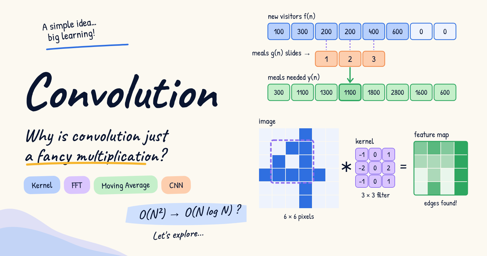
• A Trade Exhibition on community hall is registered with new visitors as [100, 300, 200, 200, 400, 600] for Monday to Saturday.
• Each registered visitor is offered 3 snack meals.
• Total Meal calculation is simple

\(\text {Total Meals count} = \text {Total Number of visitors} \space (1800) \times 3 \space meals = 5400\)

Convolution Intuition

In this case of hosting team planning, they like to upsell more products by encouraging recurring visits. They offer snacks for registered users subsequent days to their registered day.

• In addition to 3 meals on first visit day, they offer 2 meals on 2nd day and 1 meals on 3rd day for visitors.
• On Monday, they offer 3 snacks to 100 Monday visitors. \((3 \times 100)\)
• On Tuesday, they offer 3 snacks to 300 Tuesday visitors and 2 snacks to 100 Monday visitors. \((300 \times 3 + 100 \times 2)\)
• On Wednesday, they offer 3 snacks to 200 Wednesday visitors, 2 snacks to 300 Tuesday visitors, 1 snack to 100 Monday visitors. \((200 \times 3 + 300 \times 2 + 100 \times 1)\)

and so on.

Math is easy but not straightforward. right?

Let us fix the primary array in this way. - [100, 300, 200, 200, 400, 600]

and let the meal as [3, 2, 1] pass through the primary array as reversed order.

Monday:

           100, 300, 200, 200, 400, 600
 1,   2,   3
     
Total - y(0) = f(0) * g(0) = 100 * 3 = 300

Tuesday:

           100, 300, 200, 200, 400, 600
        1,   2,   3

Total - y(1) = f(0) * g(1) + f(1) * g(0) = 100 x 2 + 300 x 3 = 1100     

Thursday:

           100, 300, 200, 200, 400, 600
                  1,   2,   3

Total - y(3) = f(1) * g(2) + f(2) * g(1) + f(3) * g(2) = 300 x 1 + 200 x 2 + 200 * 3 = 1100 

For sunday and next monday, no new visitors are allowed.

Total food required on each day is

New visitor       | f(n) - [100, 300, 200, 200, 400, 600, 0, 0]

Meal              | g(n) - [3, 2, 1]

Meal on Each day  | [300, 1100, 1300, 1100, 1800, 2800, 1600, 600]

Lets set them as two functions and represent each day as expressions.

 f0,  f1,  f2,  f3,  f4,  f5
100, 300, 200, 200, 400, 600


 g0, g1, g2
  3,  2,  1
  
Monday    - y(0) = f0 * g0 = 100 * 3 = 300
Tuesday   - y(1) = f0 * g1 + f1 * g0 = 100x2 + 300x3 = 1100  
Wednesday - y(2) = f0 * g2 + f1 * g1 + f2 * g0 = 100x1 + 300x2 + 200x3 = 1300 
Thursday  - y(3) = f1 * g2 + f2 * g1 + f3 * g2 = 300x1 + 200x2 + 200x3 = 1100 

$$y(n) = (f * g) (n) = \sum_{k = -\infty}^{+\infty} f(k)\space g(n-k)$$

Thus, the overall convolution is expressed as above.

Moving Averages

We shall see the application of moving averages.

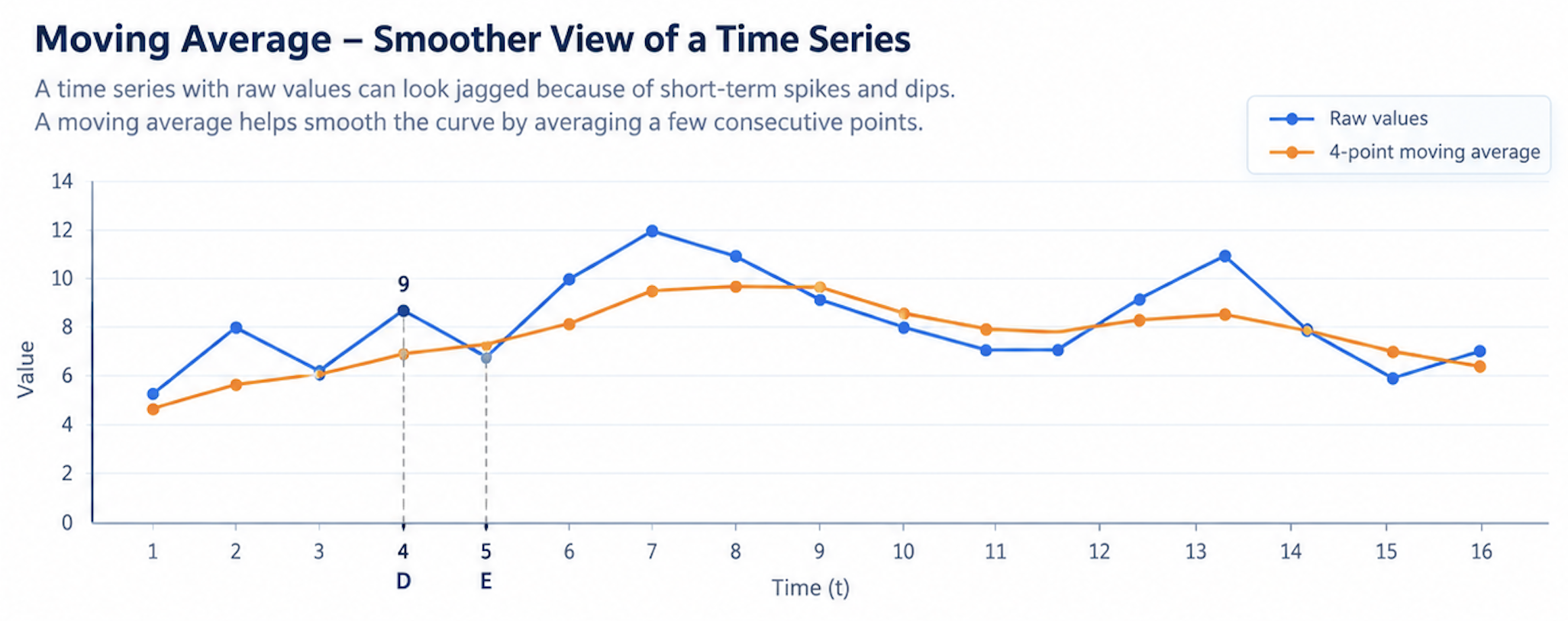
If we take any time series line graphs, discrete point of values makes the lines to take sharp turns. To make it more curvy and smooth for easy visualizations, average over time in graphs is pretty common.

In fact, many alerting system relies on it heavily to avoid frequent fluctuations between alert and safe cut-off values.

• Let us see the example. At each point in visualization, we take a series of four points (say A, B, C, D) divide them by 4.
• Calculated value will be used at the display of D. Its the not actual value at instant D. But, the average over values.
• Same applies for all instants in graphs. For next value calculation, we drop the older data (A at the instant E calculation) and take current one.

Points         -   A  B  C   D    E      F     G  
Raw Metric     -   5  6  8   9    7     10     12 
Moving Average -             7   7.5    8.5   9.5

Value at D = (5 + 6 + 8 + 9)               / 4 = 7
Value at E = (    6 + 8 + 9 + 7)           / 4 = 7.5
Value at F = (        8 + 9 + 7 + 10)      / 4 = 8.5
Value at G = (            9 + 7 + 10 + 12) / 4 = 9.5

Runtime Analysis

In Earlier Trade Exhibition example, number of mutiplication operations we did is [1, 2, 3, 3, 3, 3, 2, 1] = 18

New visitor       | f(n) - [100, 300, 200, 200, 400, 600, 0, 0]

Meal              | g(n) - [3, 2, 1]

Meal on Each day  | y(n) - [300, 1100, 1300, 1100, 1800, 2800, 1600, 600]

Operations count  | O(n) - [  1,    2,   3,   3,     3,     3,    2,   1]

Its the order O(N * M) = O (6 * 3).

For equals size of functions (N=M) its \(O(N^2)\). Its the runtime for normal convolution operation.

For larger arrays, order of N square is too costly. Thankfully, we have Convolution based on FFT (Fast Fourier transform). It has lesser runtime, O(N log N).

FFT uses domain shifting. In computations, real numbers in time domain (days) are shifted into complex numbers of frequency domain where we can use normal multiplication rather convolution.

Two list will be separately shifted to complex domain where we do normal multiplication and then, we do the InverseFFT to get back the real number values.[²]

FFT Convolution = \((f *g)(t) = IFFT (FFT(f(t)) \times FFT(g(t))\)

When we tried both approach for large array, standard convolve took 2.15 Seconds. But, fftconvolve solves it in 6.17 MilliSeconds.

In [15]: arr1 = np.random.random(100000)

In [16]: arr2 = np.random.random(100000)

In [17]: %%timeit
    ...: np.convolve(arr1, arr2)

2.51 s ± 6.38 ms per loop (mean ± std. dev. of 7 runs, 1 loop each)

In [18]: 

In [18]: import scipy.signal

In [19]: %%timeit
    ...: scipy.signal.fftconvolve(arr1, arr2)

6.17 ms ± 41.9 μs per loop (mean ± std. dev. of 7 runs, 100 loops each)

Image Processing Application

The 2-Dimension Convolution is mostly used Image processing techniques. Digital Image patterns/features can be identified and transferred easily using convolution.

• We choose 2d values (matrix) of an image as primary function f(x) .
• Function to transform the image is g(x). Its is called Kernal / Filter.
• We get the transformed matrix as output y(x). In CNN terminology, y(x) is called Convolved Feature or Activation Map or the Feature Map.[³]

Depends on whats the transformation we as output such as blur, sharpen, outline etc, we choose the respective kernel.

Edge Kernels

The small kernel/ filter like these easily extracts the features of the images when convoluted with images.[³]

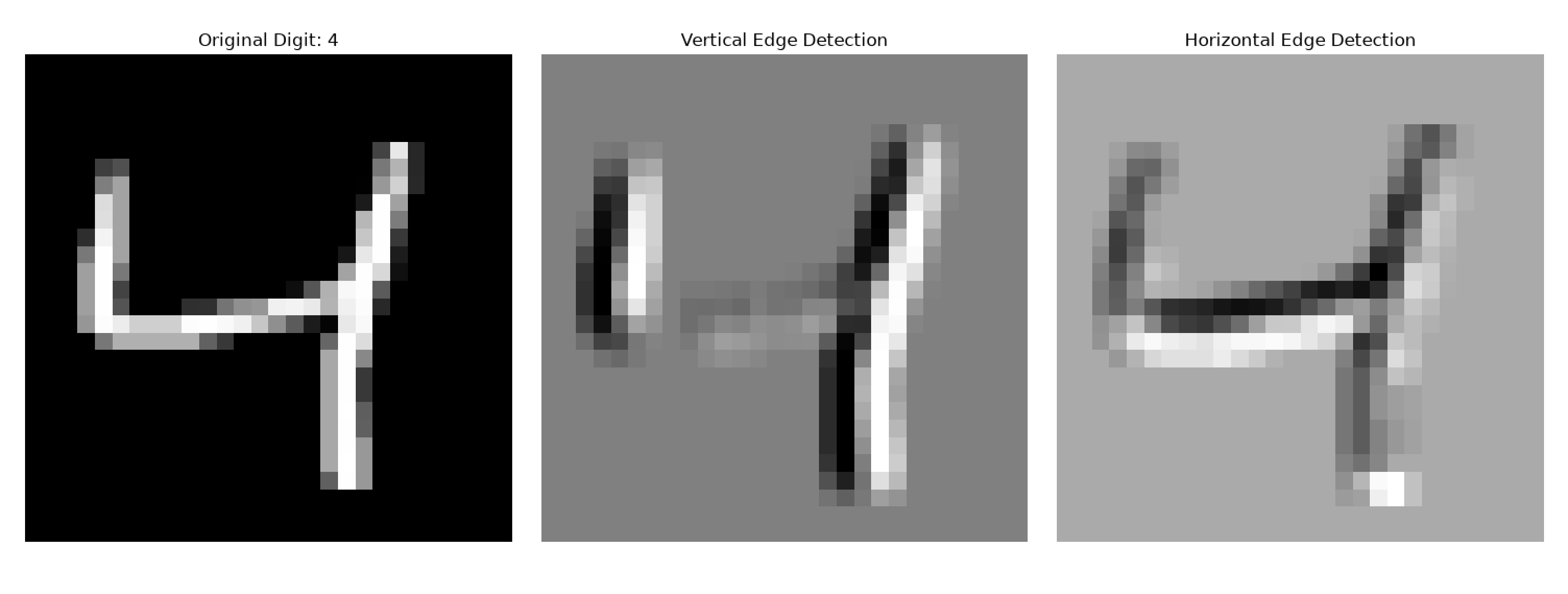
$$\text{Vertical Edge Filter} \begin{bmatrix} -1 & 0 & 1 \ -2 & 0 & 2 \ -1 & 0 & 1 \end{bmatrix} \text{Horizontal Edge Filter} \begin{bmatrix} -1 & -2 & -1 \ 0 & 0 & 0 \ 1 & 2 & 1 \end{bmatrix}$$

I've the numerical array for handwritten digit 4. Using vertical and Horizontal edge filters, we feature out the edges here.

Since everything was grayscale, tried out a photo with colors.

The Output layer has to stack the RGB layers into one array. Other steps is same as Grayscale code. Nothing fancy. we multiply image array with kernels using convolve2d function implemented in scipy package.

Here you go.

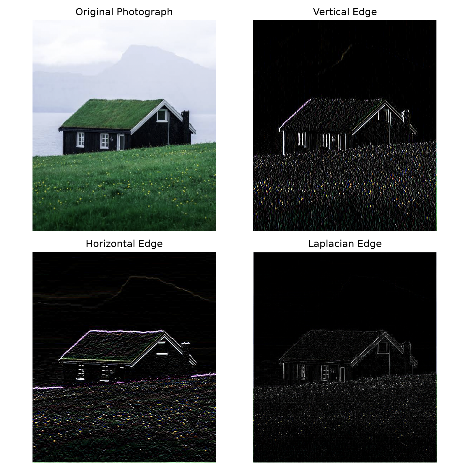
Complete code:

from PIL import Image
import numpy as np
import matplotlib.pyplot as plt
from scipy.signal import convolve2d

# Read a colored photograph
img = Image.open("blog-2/home-1.jpeg").convert("RGB")
image = np.asarray(img)

# Display the photograph and its numeric array
fig, axes = plt.subplots(2, 2, figsize=(8, 8))
axes = axes.flatten()
kernel_vertical = np.array([
    [-1, 0, 1],
    [-2, 0, 2],
    [-1, 0, 1]
])

kernel_horizontal = np.array([
    [-1, -2, -1],
    [ 0,  0,  0],
    [ 1,  2,  1]
])

kernel_laplacian = np.array([
    [ 0, -1,  0],
    [-1,  4, -1],
    [ 0, -1,  0]
])

#output_1 = convolve2d(image, kernel, mode="same", boundary="fill")
output_1 = np.stack([
    convolve2d(image[:, :, channel], kernel_vertical,
               mode="same", boundary="fill")
    for channel in range(3)
], axis=2)

output_2 = np.stack([
    convolve2d(image[:, :, channel], kernel_horizontal,
               mode="same", boundary="fill")
    for channel in range(3)
], axis=2)

output_3 = np.stack([
    convolve2d(image[:, :, channel], kernel_laplacian,
               mode="same", boundary="fill")
    for channel in range(3)
], axis=2)

axes[0].imshow(image)
axes[0].set_title("Original Photograph")
axes[0].axis("off")

axes[1].imshow(output_1, cmap="gray")
axes[1].set_title("Vertical Edge")
axes[1].axis("off")

axes[2].imshow(output_2, cmap="gray")
axes[2].set_title("Horizontal Edge")
axes[2].axis("off")

axes[3].imshow(output_3, cmap="gray")
axes[3].set_title("Laplacian Edge")
axes[3].axis("off")

plt.tight_layout()
plt.show()

History

There are multiple citations on the discovery of convolution [⁴].

Convolution is implicitly discovered as part of Laplace works of integrals. Apart from that, Its also the part of Fourier equations. While Fourier express the temperature spread over time in continuous integrals. The convolution theorem is more formalized by mathematicians after those initial discoveries. In Linear algebra, the history is much much earlier in polynomial solutions and in statistics.

There are various applications based on convolution operations in physical systems like heat transfer, Z transforms [⁵].

Conclusion

Lets wrap up. We saw Discrete convolution examples using 1-Dimension. Its application on Moving Average and Image processing. Also, the runtime improvements from \(O(N^2)\) to O(N LogN) using FFT.

Regarding Image featuring, we saw little bit about kernels and their role extracting features of image. These are building blocks in CNN architectures.

Apart from images, these CNN kernels place a big role text processing as well. We'll see CNN in detail and the role of CNN in NLP in next next blogs.

Thanks for reading.

References

Footnotes

1. https://betterexplained.com/articles/intuitive-convolution/ ↩︎

2. https://youtu.be/KuXjwB4LzSA?t=822&si=Mkwi_ggoXbP6qiRn/ ↩︎

3. https://ujjwalkarn.me/2016/08/11/intuitive-explanation-convnets/ ↩︎ ↩︎²

4. https://www.embs.org/pulse/articles/history-convolution-operation/ ↩︎

5. https://www.allaboutcircuits.com/technical-articles/dsp-applications-of-convolution-part-2/ ↩︎